Regular semisimple Hessenberg varieties · Type A

Towards the smoothness of
Hessenberg Schubert varieties

Seonjeong Park Jeonju University

Prepared for Contemporary Trends in Hamiltonian Geometry

Based on joint work:

With Soojin Cho and JiSun Huh, Towards combinatorial characterization of the smoothness of Hessenberg Schubert varieties, European J. Combin. 135, May 2026, 104353.
With Jaehyun Hong and Eunjeong Lee, Intersections of Schubert varieties and smooth T-stable subvarieties of flag varieties, arXiv:2506.21180.

When is a Hessenberg Schubert variety smooth?
We study an intersection whose smoothness can be read from its GKM graph.

Compare two examples

01 Motivation

Schubert varieties: equivalent criteria for smoothness

For an opposite Schubert variety Ω_w ⊂ Flag(ℂⁿ), geometry, topology, and combinatorics give equivalent ways to detect smoothness.

For each w ∈ 𝔖_n,

Ω_w is smooth

⇔ the GKM graph of Ω_w is regular

⇔ Poin(Ω_w) is palindromic

⇔ w avoids the patterns 2143 and 1324.

Opposite Schubert convention. For the usual X_w, the patterns are 3412, 4231.

Motivating problem

Find analogous equivalence conditions for the smoothness of Hessenberg Schubert varieties.

Goal of this talk

Find sufficient criteria for the smoothness of Hessenberg Schubert varieties by studying intersections of Hessenberg varieties with Schubert varieties.

Background: the two varieties we need to distinguish

Fix a diagonal matrix S with pairwise distinct eigenvalues and a Hessenberg function h : [n] → [n], with i ≤ h(i) and h(i) ≤ h(i+1) whenever the terms are defined.

The intersection

Ω_w ∩ Hess(S,h)

Intersect the entire opposite Schubert variety with Hess(S,h).

The Hessenberg Schubert variety

Ω_w,h = $Ω_{w}^{○}$ ∩ Hess(S,h)

Take the closure of the intersection with the opposite Schubert cell.

In general, Ω_w,h is an irreducible component of Ω_w ∩ Hess(S,h), and this intersection can be reducible. Even when their fixed-point sets coincide, their GKM graphs can have different edges. See the graph comparison below.

From flags to graph edges: the construction and its formulas ↓

The graph behind the criterion

The GKM graph of $Hess (S, h) \cap Ω_{w}$

Let $S$ be diagonal with pairwise distinct eigenvalues, and let $T$ be the diagonal torus. The regular semisimple Hessenberg variety $Hess (S, h)$ is a smooth GKM variety, and the intersection $Hess (S, h) \cap Ω_{w}$ is also GKM. The GKM graph of this intersection is the subgraph of the ambient Hessenberg graph induced by its $T$ -fixed point set, identified with the Bruhat interval $[w, w_{0}]$ .

01Description: vertices, edges, and labels

01 · The ambient Hessenberg graph

$Γ_{h} = Γ (Hess (S, h))$

Vertices

V (Γ_{h}) = {Hess (S, h)}^{T} = 𝔖_{n}

Edges

E (Γ_{h}) = {{u, u (i, j)} : u \in 𝔖_{n}, 1 \leq i < j \leq h (i)}

Labels, up to sign

α ({u, u (i, j)}) = \pm (t_{u (i)} - t_{u (j)})

The transposition $(i, j)$ swaps positions. The label records the two swapped values. Each edge represents a $T$ -stable curve.

02 · Restrict to the Bruhat interval

The graph of the intersection

Keep the fixed points above $w$

{(Ω_{w} \cap Hess (S, h))}^{T} = [w, w_{0}]

Take the induced subgraph

Γ (Ω_{w} \cap Hess (S, h)) = {Γ_{h} |}_{[w, w_{0}]}

Here the restriction symbol means induced subgraph: keep every edge of $Γ_{h}$ whose two endpoints lie in $[w, w_{0}]$ . The edge labels are inherited.

Equivalently, retain the edge ${u, u (i, j)}$ exactly when

$1 \leq i < j \leq h (i)$ , and
$u \geq w and u (i, j) \geq w$ .

The two inequalities are in Bruhat order. This graph construction works for every $w \in 𝔖_{n}$ , without an admissibility assumption.

Two filters, in order:

h

selects allowed position swaps;

w

selects the Bruhat interval. This constructs the graph of

Ω_{w} \cap Hess (S, h)

, not automatically the graph of its component

Ω_{w, h}

Why is this a GKM variety?

The fixed points are the finitely many coordinate flags, and the one-dimensional torus orbits are inherited from the flag variety. The affine paving

Hess (S, h) = ⨆_{u \in 𝔖_{n}} (Ω_{u}^{○} \cap Hess (S, h))

has cells of dimension $d_{h} - ℓ_{h} (u)$ . Thus odd cohomology vanishes, giving equivariant formality. Restricting this paving to $u \geq w$ gives the GKM description of the intersection.

Hong–Lee–Park, Proposition 2.2 and the paving (p. 7); equation (2.4) and the induced subgraph (p. 8). Cho–Huh–Park, Proposition 2.5.

Graph formulas: Hong–Lee–Park, Proposition 2.2 and p. 8, in the supplied revision dated 20 September 2026.

02Example: filter edges, then vertices

A small construction example · n = 3

Filter edges, then vertices

Hessenberg function Schubert index

Intersection graph

4 vertices · 3 edges

Keep the vertices u ≥ 213 in Bruhat order and the Hessenberg edges between them.

Select a vertex

Click a retained vertex to inspect its incident edges.

Dashed gray edges and pale vertices are removed by the filters. The vertical levels show ordinary Coxeter length; color does not mark singularities.

02 Main result

Smoothness criterion for the intersection Ω_w ∩ Hess(S,h)

Let w be h-admissible. The following conditions are equivalent.

IGeometry
Ω_w ∩ Hess(S,h) is smooth.
IIGraph
Γ(Ω_w ∩ Hess(S,h)) is regular: every vertex has the same degree.
IIITwo endpoints
deg(w₀) = deg(w) = d_h − ℓ_h(w).
IVTopology + geometry
Ω_w ∩ Hess(S,h) is irreducible and its Poincaré polynomial is palindromic.
VPatterns
w avoids the seven associated h-patterns.
See the precise conditions

Two proof ingredients: the key lemma for (2)–(5) and the type-A tangent-space input for (2) ⇒ (1).

When these conditions hold

Ω_w ∩ Hess(S,h) = Ω_w,h and Ω_w,h is smooth.

For arbitrary w, apply the criterion to its h-admissible representative w̃. This gives sufficient conditions for Ω_w,h to be smooth. The converse fails.

Hong–Lee–Park, current manuscript: Theorems 1.2–1.3 and 4.7, Corollary 4.6. Read the statements ↗
Cho–Huh–Park, European J. Combin. 135 (2026), 104353: Theorem C(1), the seven-pattern criterion ↗.

Hypotheses and notation

Throughout: type A over ℂ, with S regular semisimple and diagonal. The graph Γ is the GKM graph of the intersection Ω_w ∩ Hess(S,h). For admissible w, it is connected. For an arbitrary permutation, Theorem 1.2 assumes connectedness before asserting regularity ⇔ smoothness.

$d_{h} = \sum_{i = 1}^{n} (h (i) - i)$

ℓ_h(v) = #{(i,j) : i < j ≤ h(i), v(i) > v(j)}

w₀ = n⋯21 is the longest permutation. Graph degree means the number of incident edges.

03 Interactive examples · Flag(ℂ⁴)

Smooth and singular intersections

Keep h = (3,3,4,4) fixed. Change w, rotate the graph, and select a vertex to inspect its degree.

Drag to rotate; use + / − to zoom. Select a vertex, or use ← / → inside the graph. Red marks degree above d_h − ℓ_h(w); gold marks admissible permutations. The 3D height does not represent an order.

Open the full graph explorer ↗

Why the converse fails · Hong–Lee–Park, Example 5.5

A singular intersection can contain a smooth Hessenberg Schubert variety.

For h = (3,3,4,4), w = 2134, the two graphs have the same 18 vertices. The graph of Ω_2134,h has three fewer edges and is 3-regular. The manuscript proves that this Hessenberg Schubert variety is smooth.

Edges present only in the intersection

2341 — 4321
3241 — 4231
2431 — 3421

Source: Hong–Lee–Park, Example 5.5, pp. 21–22 (20 September 2026 revision); Figure 5, p. 22. Explore the component and its boundary below ↓

Choose any of the 14 functions and 24 permutations in 𝔖₄

Hessenberg function Permutation Show only h-admissible permutations

These controls always display the full intersection graph. For a disconnected graph, the connectedness hypothesis of Theorem 1.2 is unavailable; no smoothness conclusion is inferred here.

Inspect all vertex degrees and the intersection’s Poincaré polynomial

P(q) = 1 + 2q + 2q² + q³

For the intersection: P_w,h(q) = ∑_{v ≥ w} q^{d_h − ℓ_h(v)}, where q has cohomological degree 2. The coefficient counts cells of the corresponding complex dimension.

3D graph explorer originally created by Eunjeong Lee with the help of GPT. Adapted here with guided examples, degree readouts, and the manuscript’s component comparison.

04 Key lemma

Degrees increase along
the h-Bruhat order.

Where this lemma is used. The injection and degree monotonicity underpin the arguments relating conditions (2)–(5). The implication (2) ⇒ (1) needs an additional geometric input: the type-A tangent-space equality. See the two roles and the smoothness proof ↓

Fix an h-admissible w. In the intersection graph, an increasing path of allowed transpositions has nondecreasing vertex degrees.

u ≤_h v ⟹ deg(u) ≤ deg(v)

Every vertex lies between w and w₀ in this order. Thus equal endpoint degrees force every degree to agree.

Why two endpoints suffice

deg(w) ≤ deg(v) ≤ deg(w₀)

The minimum is d_h − ℓ_h(w). Compare it with deg(w₀) to test regularity.

Try an increasing path for h = (3,3,4,4), w = 2134. Each step selects the vertex in the graph above.

(2,3)
→(3,4)
→(1,3)
→

The labels on the arrows are swaps of positions. These are increasing h-edges; they need not be cover relations.

What is h-Bruhat order, and why does the lemma hold?

The h-Bruhat order is the transitive closure of u <_h u(i,j) with 1 ≤ i < j ≤ h(i) and ℓ(u(i,j)) > ℓ(u).

The incident-edge injection

For a vertex u of Γ(Ω_w ∩ Hess(S,h)), set

E_w,h(u) = {(i,j) : 1 ≤ i < j ≤ h(i), u(i,j) ≥ w}.

Let v = u(a,b) be joined to u by an increasing h-edge. Define φ_uv : E_w,h(u) → E_w,h(v) by

φ_uv(i,j) =

(b,j)if i=a, j>b, and (b,j) ∉ E_w,h(u),

(i,a)if i<a, j=b, and (i,a) ∉ E_w,h(u),

(i,j)otherwise.

Both non-membership tests refer to the source set E_w,h(u). The map is almost the identity; it changes a position pair only in these two exceptional cases.

Cho–Huh–Park, Lemma 3.7. If w is h-admissible, this map is well-defined and injective. Consequently, deg(u) ≤ deg(v).

Example 3.6(2) · a changed pair

3124 → 3214 = 3124(2,3)

h = (3,3,4,4), w = 2134
At 3124	At 3214
(1,3)	(1,2)
(2,3)	(2,3)
(3,4)	(3,4)

The injection is a bijection. Both degrees are 3.

Example 3.6(1) · a missed edge

2314 → 2341 = 2314(3,4)

h = (3,3,4,4), w = 2134
At 2314	At 2341
(1,2)	(1,2)
(2,3)	(2,3)
(3,4)	(3,4)
No preimage	(1,3)

The injection is not surjective. The degree increases from 3 to 4.

Cho–Huh–Park, Lemma 3.7 (p. 12) ↗ · Definition of the map (p. 11) · Theorem 3.8 (p. 13)

Two ingredients in the main theorem

From graph regularity to smoothness

Degree monotonicity organizes the combinatorial and topological criteria. To pass from (2) a regular graph to (1) a smooth intersection, we must also control the entire tangent space.

Combinatorial input · conditions (2)–(5)

The incident-edge injection

φ_{u v} : E_{w, h} (u) ↪ E_{w, h} (v)

For an increasing $h$ -edge, the injection gives $\deg_{Γ} (u) \leq \deg_{Γ} (v)$ . It is used in three ways:

(2) ⇔ (3)

The bounds $\deg_{Γ} (w) \leq \deg_{Γ} (v) \leq \deg_{Γ} (w_{0})$ reduce regularity to equality of the endpoint degrees.

Cho–Huh–Park, Theorem 3.8 (p. 13).

(4) ⇒ (2)

Irreducibility and palindromicity give average degree $d = d_{h} - ℓ_{h} (w)$ . The lower bound $\deg_{Γ} (v) \geq d$ then forces every degree to be $d$ .

Hong–Lee–Park, Theorem 4.7 (p. 15).

(2) ⇔ (5)

Forbidden $h$ -patterns produce injections that are not surjective. The converse uses additional pattern-avoidance and inductive arguments; it does not follow from injectivity alone.

Cho–Huh–Park, Theorem C(1): Theorem 3.12 (p. 15) and Theorem 4.9 (p. 23).

Geometric input · (2) ⇒ (1)

The type-A tangent-space equality

For every $v \in {Ω_{w}}^{T}$ ,

T_{v} (Ω_{w}) = TE (Ω_{w}, v)

Here

TE (V, v) := \sum_{C \in E (V, v)} T_{v} C

and $E (V, v)$ is the set of $T$ -stable curves in $V$ through $v$ . Thus every tangent direction of a type-A Schubert variety is spanned by directions of these curves.

Since $Hess (S, h)$ is smooth, we also have

T_{v} (Hess (S, h)) = TE (Hess (S, h), v)

Why this matters: graph degree counts curve directions. These equalities let us identify those directions with the full tangent space of the intersection.

Type-A equality: Lakshmibai–Seshadri, Theorem 1, as cited in Hong–Lee–Park, p. 2.

The geometric step: at a fixed point, intersect the two spaces of curve directions. The ambient GKM weight-space decomposition identifies their common directions with the curves lying in both varieties.

Why (2) implies (1)

Assume $w$ is $h$ -admissible, and that $Γ = Γ (Ω_{w} \cap Hess (S, h))$ is regular. The graph is connected. Set

d = \dim Ω_{w, h} = d_{h} - ℓ_{h} (w) = \deg_{Γ} (w)

Step 1 · Propagate along the graph

The affine cell at $w$ is open in the intersection and is smooth of dimension $d$ , so the common degree is $d$ . Proposition 3.4 shows that every vertex $v$ belongs to $Ω_{w, h}$ and that the incident curves of this component agree with those of the intersection.

This gives a $d$ -dimensional component through every fixed point. Equality of the two graphs is not being used by itself to assert equality of the varieties.

Step 2 · Use the tangent-space equalities

At every fixed point $v \in [w, w_{0}]$ ,

TE (Ω_{w} \cap Hess (S, h), v)

\subseteq T_{v} (Ω_{w} \cap Hess (S, h))

\subseteq T_{v} (Ω_{w}) \cap T_{v} (Hess (S, h))

= TE (Ω_{w}, v) \cap TE (Hess (S, h), v)

= TE (Ω_{w} \cap Hess (S, h), v)

The first inclusion comes from curves in the intersection; the second is the tangent-space inclusion for an intersection. The two equalities use the type-A result, smoothness of $Hess (S, h)$ , and the distinct weight lines of the ambient GKM tangent space.

T_{v} (Ω_{w} \cap Hess (S, h)) = TE (Ω_{w} \cap Hess (S, h), v)

\dim T_{v} (Ω_{w} \cap Hess (S, h)) = \deg_{Γ} (v) = d

Step 3 · Compare local and tangent dimensions

By Step 1, $v$ lies in the component $Ω_{w, h}$ of dimension $d$ . Therefore,

d \leq \dim_{v} (Ω_{w} \cap Hess (S, h)) \leq \dim T_{v} (Ω_{w} \cap Hess (S, h)) = d

The intersection is smooth at every fixed point. A nonempty singular locus would be closed, projective and $T$ -stable, and hence would contain a fixed point. Thus the intersection is smooth everywhere. Connectedness then gives

Ω_{w} \cap Hess (S, h) = Ω_{w, h}

Proof: Proposition 3.4, pp. 10–11, and proof of Theorem 1.1, p. 11. Connectedness for admissible $w$ : Proposition 4.1.

How the average-degree argument uses the key lemma

Under condition (4), irreducibility makes the dimension of the cell at $w$ the degree $d$ of $P_{w, h} (q)$ . Palindromicity and the affine paving give

P_{w, h} (1) = | V (Γ) |, P_{w, h}^{'} (1) = | E (Γ) |

d | V (Γ) | = 2 | E (Γ) |

Thus the average degree is $d$ . Monotonicity gives $\deg_{Γ} (v) \geq \deg_{Γ} (w) = d$ at every vertex, so all degrees must equal $d$ . Irreducibility cannot be dropped: a different component may have larger dimension, changing the degree of the Poincaré polynomial.

Hong–Lee–Park, Theorem 4.7 and Example 4.8.

Sources and attribution

The supplied revision cites Lakshmibai–Seshadri, Theorem 1 for $T_{v} (Ω_{w}) = TE (Ω_{w}, v)$ . It cites Carrell separately for the lower bound on the number of $T$ -curves through a fixed point (Lemma 3.3), which is used in the propagation argument.

Introduction, p. 2 · Lemma 3.3, p. 10 · References [4] and [12], p. 23.

05 Go further

Three details behind the criterion.

01 Why it is enough to study h-admissible permutations

A permutation w is h-admissible if

w⁻¹(w(j) + 1) ≤ h(j) whenever w(j) < n.

Every permutation has a unique h-admissible representative w̃ ≥ w with the same relative comparisons on the allowed position pairs:

w̃(i) < w̃(j) ⇔ w(i) < w(j), i < j ≤ h(i).

The associated Hessenberg Schubert varieties are related by a permutation of coordinates, allowing a conjugate regular semisimple matrix. This transports the smoothness criterion back to the original Ω_w,h.

Example 5.3 · h = (3,3,4,4)

3214 has admissible representative 4312.

The original intersection has 8 vertices and 9 edges. Its Hessenberg Schubert variety has just the edge 3214 — 3241. The representative’s intersection is the edge 4312 — 4321, so the criterion applies.

The precise geometric relation

Set a = w w̃⁻¹. Proposition 2.5 gives

Ω_w,h = a · $Ω_{w̃}^{○}$ ∩ Hess(a⁻¹Sa,h).

This statement concerns closures of cells. It does not identify the original intersection Ω_w ∩ Hess(S,h) with the representative’s intersection.

Definition 2.3 and Proposition 2.5 ↗

02 Why “irreducible” is part of the palindromicity condition

Let d = d_h − ℓ_h(w). For irreducible Ω_w ∩ Hess(S,h), its Poincaré polynomial has degree d. Palindromicity then implies

2P′(1) = dP(1).

Since P(1) = |V| and P′(1) = |E|, the average graph degree equals d. The degree lemma says every degree is at least d. Consequently every degree is exactly d.

Example 4.8 · an essential hypothesis

A palindromic polynomial with a singular intersection.

h = (2,4,5,5,5), w = 12534 is admissible, and

P(q) = 1 + 8q + 27q² + 27q³ + 8q⁴ + q⁵.

1q⁰

8q¹

27q²

27q³

8q⁴

1q⁵

Yet deg(w) = 4 and deg(w₀) = 6. The graph is not regular, and the intersection is reducible and singular. Its 72 vertices split equally among degrees 4, 5, and 6.

This example is in Flag(ℂ⁵); the 3D explorer above is restricted to Flag(ℂ⁴).

Theorem 4.7 and Example 4.8 ↗

03 The seven associated h-patterns: the role of h

An associated h-pattern has two tests: the relative order of the selected values, and the graph determined by h on the selected positions. An ordinary occurrence can fail the second test.

1 · Value order matches the permutation patternAND2 · Position graph matches one of its allowed shapes

Figure 4: the seven associated patterns and their permitted induced graphs on positions i,j,k,ell — Cho–Huh–Park, Fig. 4. The permitted induced subgraphs of inc(h) on {i,j,k,ℓ}. View the source (p. 14) ↗ · Select the figure to enlarge it.

What can h rule out before looking at w?

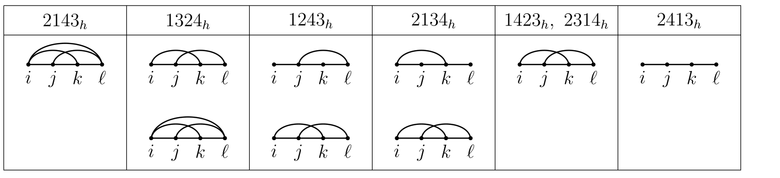
For a fixed h, a pattern is automatically excluded if no four positions satisfy its graph condition. “Possible” below means only that the positions can support the pattern; the selected values still have to match.

Compare Hessenberg functions

Inspect a pattern

2143ₕ

ℓ ≤ h(i)

Among these four entries, the relative ranks are 2, 1, 4, 3.

Relative ranks alone do not determine an associated pattern. The selected positions must also induce an allowed graph in inc(h).

Cho–Huh–Park · Example 3.10

The same value pattern need not be an h-pattern

h = (3,5,6,6,6,7,8,8), w = 27318456

Variation only: change h(5) from 6 to 7

The published example uses h(5) = 6. The switch changes h, not the permutation or selected positions.

Ordinary pattern · value test

Induced graph · position test

Check the h-dependent inequalities
Condition	Values in this example	Holds?

Source: Example 3.10 (p. 14) and Fig. 5 (p. 15). The h(5) = 7 case is an explicitly labeled variation.

Complete list of associated patterns
Pattern	Additional conditions
2143_h	ℓ ≤ h(i)
1324_h	ℓ ≤ h(j), k ≤ h(i)
1243_h	ℓ ≤ h(j), j ≤ h(i) < ℓ
2134_h	ℓ ≤ h(k), k ≤ h(i) < ℓ
1423_h	ℓ ≤ h(j), k ≤ h(i) < ℓ
2314_h	ℓ ≤ h(j), k ≤ h(i) < ℓ
2413_h	j ≤ h(i) < k ≤ h(j) < ℓ ≤ h(k)

Exact definitions: Cho–Huh–Park, Definition 3.9 (pp. 13–14). Automatic avoidance: full-flag case (p. 4) and Remark 3.11 (p. 14).

06 Towards the motivating problem

Beyond the intersection criterion

The sufficient criterion is now in place. To seek an equivalence for Ω_w,h itself, we need to understand the geometry of the component, not only that of Ω_w ∩ Hess(S,h).

Questions for discussion, with examples from the supplied papers. The affine-paving and curve-detection questions below are research directions, not conclusions of the main theorem.

01 · Cells and cohomology

Does Ω_w,h admit an affine paving?

The ambient Hess(S,h) and the full intersection have affine pavings. Their affine cells do not automatically provide a paving of one irreducible component by whole ambient cells.

Ω_{w, h} = ⨆_{v \in Ω_{w, h}^{T}} (Ω_{w, h} \cap Ω_{v}^{○})

Describe these pieces: are they affine spaces, or can they be refined into an affine paving? The general, possibly singular, closure is the case to investigate.

A three-dimensional cell meets the component in a two-dimensional slice ↓

Ambient and intersection pavings: Hong–Lee–Park, (2.3), p. 7, and (2.4), p. 8.

02 · Fixed points and curves

Which edges belong to the component?

Knowing the torus fixed points gives a candidate induced graph. A curve joining two of those points need not lie in Ω_w,h.

Γ (Ω_{w, h}) \subseteq {Γ (Hess (S, h)) |}_{Ω_{w, h}^{T}}

Find a combinatorial test, in terms of w, h, v and (i,j), for the corresponding T-stable curve to be contained in Ω_w,h.

Same 18 fixed points, but three curves are missing ↓

The graph of fixed points and actual T-curves is the one-skeleton. Equivariant formality must also be established to use the full GKM cohomology description. See §3 and Remark 4.10.

One example, two distinctions

Hong–Lee–Park, Example 5.5

h = (3,3,4,4), w = 2134, S = diag(1,2,3,4).

Section 5 · pp. 21–22 ↗
Figure 5 · p. 22 ↗Revision dated 20 September 2026

This is the same example used in the interactive comparison above: Ω_2134,h is smooth, although Ω₂₁₃₄ ∩ Hess(S,h) is reducible and singular.

Boundary slice: an affine plane inside an ambient affine 3-space

In the chart at v = 2341, the ambient cell $Ω_{2341}^{○}$ ∩ Hess(S,h) is given by

x_{41} = x_{42} = x_{43} = 0

Its free coordinates are x₂₁, x₃₁, x₃₂. Restricting the local ideal of Ω_2134,h to this cell leaves the additional equation

3 x_{32} \cdot x_{21} - 4 x_{31} = 0

x₂₁Free coordinate

x₃₁Free coordinate

x₃₂Free coordinate

The ambient cell is 𝔸³: all three coordinates vary independently.

The distinction: the component contains a proper slice of the ambient cell, not the whole cell. A description of the component's pieces must account for these extra equations.

This slice computation is obtained by restricting the local ideals in Example 5.5, p. 22. It is not a counterexample to affine paving: this component is smooth. The example explains why taking a union of whole ambient cells is not the general answer.

The actual one-skeleton: 30 edges in the intersection, 27 in the component

Both varieties have the same 18 fixed points. The intersection graph has 30 edges; the actual graph of Ω_2134,h has 27. The following three edges belong only to the intersection:

2341 — 43213241 — 42312431 — 3421

A local explanation for one missing curve. At 2341, the curve towards 4321 = 2341(1,3) is the x₃₁-axis in this chart. On this axis, the component equation 3x₃₂x₂₁ − 4x₃₁ = 0 forces x₃₁ = 0. Thus the component contains the fixed point, but not this curve.

Even for an h-admissible permutation, the induced graph on the fixed points can therefore be larger than the actual component graph. The research task is to replace such chart-by-chart tests with a combinatorial rule.

The three deleted edges are listed in Example 5.5 and Figure 5, p. 22. The axis test is a direct check using the same chart and local ideal. Return to the original graph comparison ↑

A related task: identify the irreducible components

Question 5.1 asks for explicit component descriptions. In Example 5.3, for h = (3,3,4,4), the manuscript gives

Ω_{3214} \cap Hess (S, h) = Ω_{3214, h} \cup Ω_{3412, h} \cup Ω_{3241, h} \cup Ω_{4213, h}

The component Ω_3214,h is a curve, whereas Ω_3412,h has dimension 2. The full intersection is therefore not equidimensional. Identifying the desired component is an important first step before computing its cells or curves.

Hong–Lee–Park, Question 5.1 and Example 5.3, pp. 20–21. Compare the admissible representative example ↑

Back to the motivating problem

Can the component's cells, actual curves, and tangent spaces be described combinatorially, and then used to characterize the smoothness of Ω_w,h?

The original smoothness question is Hong–Lee–Park, Question 5.4. A regular one-skeleton alone should not be treated as an established sufficient criterion for an arbitrary component; the tangent-space step still needs justification.

Schubert varieties: equivalent criteria for smoothness

The GKM graph of Hess(S,h)∩Ωw

01Description: vertices, edges, and labels

Γh=Γ(Hess(S,h))

The graph of the intersection

02Example: filter edges, then vertices

Filter edges, then vertices

4 vertices · 3 edges

Smoothness criterion for the intersection Ωw ∩ Hess(S,h)

Smooth and singular intersections

A singular intersection can contain a smooth Hessenberg Schubert variety.

Degrees increase alongthe h-Bruhat order.

The incident-edge injection

From graph regularity to smoothness

The incident-edge injection

The type-A tangent-space equality

Three details behind the criterion.

3214 has admissible representative 4312.

A palindromic polynomial with a singular intersection.

What can h rule out before looking at w?

Inspect a pattern

2143ₕ

The same value pattern need not be an h-pattern

Beyond the intersection criterion

Does Ωw,h admit an affine paving?

Which edges belong to the component?

Hong–Lee–Park, Example 5.5

The GKM graph of $Hess (S, h) \cap Ω_{w}$

$Γ_{h} = Γ (Hess (S, h))$

Smoothness criterion for the intersection Ω_w ∩ Hess(S,h)

Degrees increase along
the h-Bruhat order.

Does Ω_w,h admit an affine paving?